The Game of Mill: Instructions

User Manual

This page serves as a comprehensive manual for users, explaining what the software can do, and how to use it. Its contents are arranged in a sequence matching the arrangement on the Game Page where you can play the game. You can read the manual as an introductory (and spell-binding!) narrative. You can also click on any item in this table of contents to get to any particular spot. If you see a link like this ↩ you can click on it to get back to the list of contents. Also keep in mind that you can hover over any component of the game page and see an explanatory window pop up after a couple of seconds.

The computer algorithm	The game page	The system clock	The game board
Status window and console	Selecting players	Move and board scores	Playing at random
Graphical aids	Collecting data	Parallel processing	Increasing efficiency
AI players	Static evaluations	Silence is golden	Dealing with brains
Modifying a brain	Brain improvement	Import/export brains	Running a tournament
Setting up a board	Switching engines	Playing and resetting	The game table

The computer algorithm ↩

A rudimentary understanding of how the computer plays is useful for understanding how to use the controls. For more detailed information a complete description of the algorithm is available. Here is an extremely terse introduction: The moves available to the computer form a tree rooted at the current board position. The computer examines that tree to a certain depth. It uses a formula (the static evaluation) to assign a value to each relevant leaf of the tree. It then determines which best static value the player can obtain with perfect play, and makes the required move. The depth of computer searches can be fixed or vary widely if limited by the game clock.

There are many references to time on this page. A JavaScript code running in a browser has no facility to measure the amount of time used by the CPU, and in any case, the concept of CPU time becomes ambiguous when using parallel processes. All times in these notes are elapsed wall-clock time, but care was taken to ensure that they are measured only when the computer was essentially doing nothing but running the Mill software, and the browser window was at least partially visible on the screen. As a result, those stated times are reasonably comparable and reproducible on the particular machine they were obtained.

The following Table illustrates the performance of the computer algorithms on my particular Windows 11 machine. The software offers two engines, one written in JavaScript (JS), and one written in C++. The C++ version is much faster than the JS version. However, while the JS version works with essentially any browser, the C++ engine may not work on your particular computer. It requires a compiled version of the C++ code that is part of the package.

There are two blocks in the Table, the first one corresponding to the C++ engine, the second corresponding to the JS version. The Table shows data for a computation of the first move (with the opening book being turned off). The main columns go with the depth of the computer search. That depth is measured in plies, i.e., half moves. A move consists of a ply performed by White, followed by a ply performed by Black. The row headed Nodes gives the number of nodes of the tree visited by the code for this particular depth. This number is only a little larger than the number of leaves where the static evaluation is performed. The next row gives the Time measured in milliseconds (ms). The third row of each block, Nodes/Time, gives the number of nodes that were visited each millisecond. The row labeled Time Factor gives the ratio of the time for the current depth and the time for the preceding depth. It is a measure of the branching factor, i.e., the average number of nodes attached to a single node two levels higher in the tree.

Metric	Engine	Depth 2	Depth 4	Depth 6	Depth 8	Depth 10	Depth 12
Nodes	C++	96	5,859	622,771	11,044,969	158,178,627	3,585,455,835
Time (ms)	C++	12	14	63	824	12,090	283,492
Nodes/Time	C++	8	419	9,886	13,404	13,084	12,648
Time Factor	C++		1	4	13	15	23

Nodes	JS	96	5,859	619,556	10,515,717	116,666,470	2,118,151,527
Time(ms)	JS	14	33	445	7,813	141,598	27,562,078
Nodes/Time	JS	7	178	1,393	1,346	824	77
Time Factor	JS		2	13	18	18	195

Time	JS/C++	1	2	7	9	12	97

It is evident that the C++ engine is significantly faster than the JS engine, by a typical factor 10. The initial factors 1 and 2 are not significant because the times involved are mostly determined by overhead. For depth 12 the JS engine technically succeeds in computing the move, but it is virtually useless since it takes almost 8 hours for the calculation. The reason why C++ is generally faster is that it is a compiled language while JS is interpreted. The basic reason why JS fails at depth 12 is that C++ has a much more efficient way than JS of handling arrays, and JS runs into memory limitations at that stage.

Note that the complexity of the game tree varies greatly with the board state. After all pieces are on the board, and many are blocked, the branching factor in the tree is much smaller, and a given depth requires less time. This is clearly visible if you play a game with time (rather than depth) controls. In the middle game the computer will do a much deeper search than earlier in the game.

The game page ↩

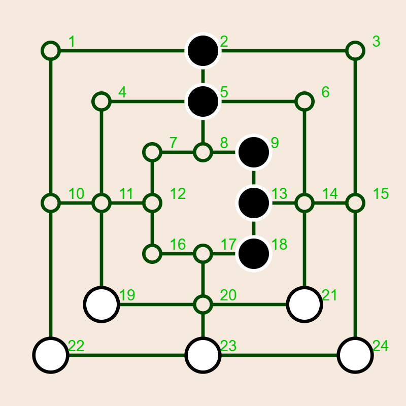
To understand the following discussion of the game controls it is best to bring up the actual game page in a different window, but you can also use this static image:

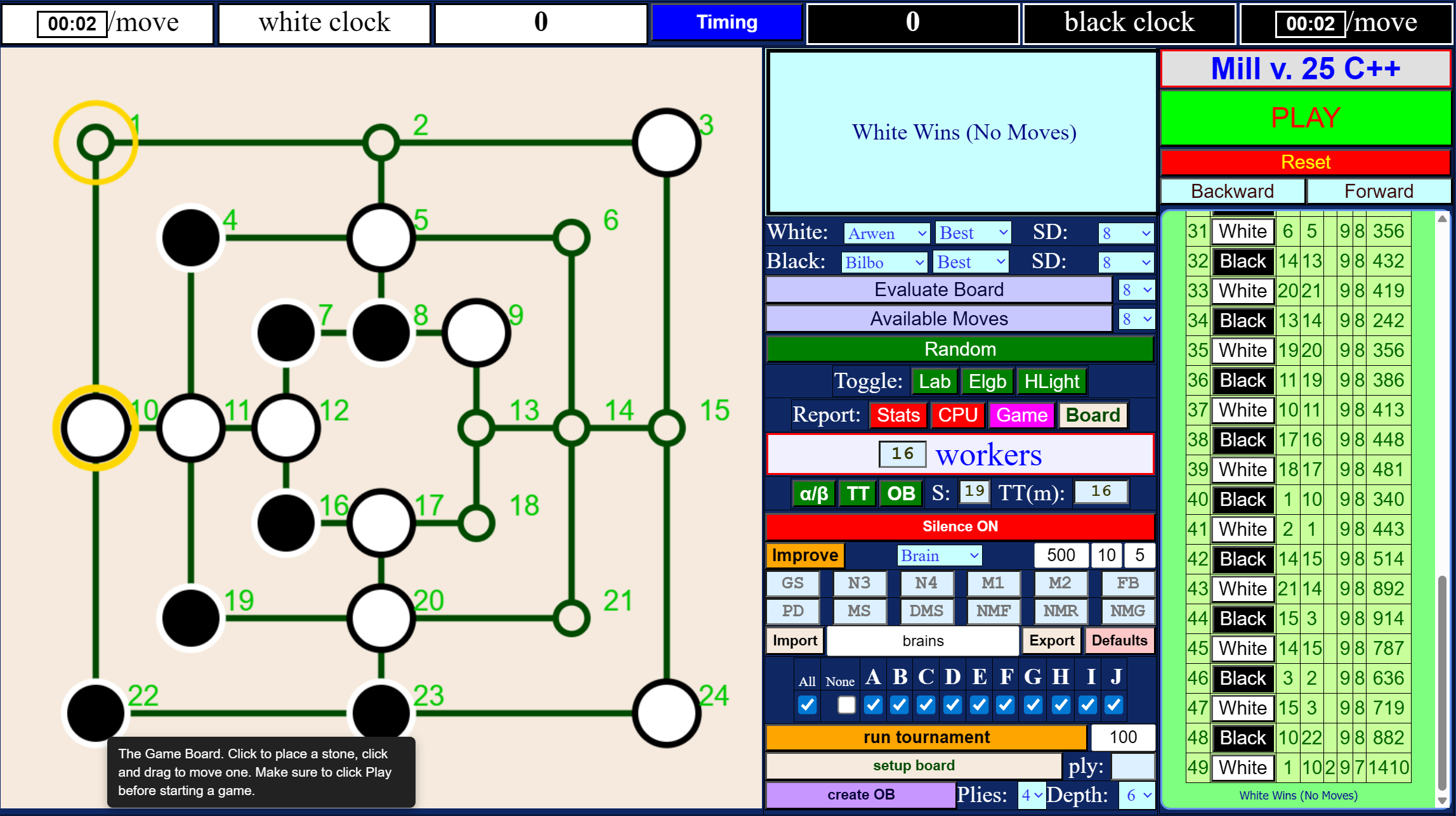
The image shows the game table on the the game page where you can play a game or otherwise explore this software. You can get to it by clicking on the image, by clicking on the small board in the headline of any of these pages, or right here. The contents of the game page (the table with the board and the controls, plus the row of links below the table) take up a space of approximately 1330 pixels wide by 910 pixels high. Most laptops and desktops can accommodate that space. However, depending on your settings, you may find it convenient to adjust the resolution of your display. Notice the Black box with explanatory text at the bottom of the game board. All the controls in the game table have a box like that attached to them that will pop up after two seconds if you hover over that control with your mouse. The box will disappear when you move the mouse elsewhere.

If you are are not familiar with the game of mill there is a page with game rules here.

The particular image above shows the window after a match between Arwen and Bilbo, two of the built-in AI personalities. Arwen (playing White) won after 49 plies (half moves) by blocking Bilbo so that he was unable to make another move.

The system clock ↩

The top row of the game table contains the system clock which works much like an ordinary chess clock. Its main purpose is to govern variable depth computer play, but it can also be used by human players. The left side of the clock (text fields with White backgrounds) constitutes the White clock, the right side the Black clock. In the center is the Timing Button which activates the clock for human players.

The key parameter for the clock is the time interval that can be set separately for White and Black. When it is the computer’s move it will start by searching for the best move at a depth of 2 plies (one move). At the end of the search it will take note of the best move it found. It will then increase the current search depth by 2 and start a new search. This process is repeated until more than 2% of the available time has passed after concluding the search at the current depth. The required search time increases greatly with the search depth, which is the reason for starting a new search only within a very short time interval at the beginning of the available time. The default time interval is 2 seconds. It happens rarely, but it is possible that the system runs out of time and loses, despite the precautions, particularly at very short time intervals when overhead becomes more significant. The maximum search depth varies greatly with the available time, and the state of the game board. There is no formal upper bound on the search depth. In practical play on a common PC typical search depths range from 4 to 16 or so. The time available for a move will increase with the first few moves and in long games will stabilize around 10 or 20 times the length of the time interval.

A typical time for a search depth of 8 is less than a second, whereas for a search depth of 10 it may be a significant fraction of a minute. The system can technically search at depth 20, but it would take you several years to see the answer.

Note that the system clock measures wall-clock time. This puts a computer brain at a disadvantage when the system is busy with heavy computational tasks, or running in the background. For example, if you wish to improve several computer brains simultaneously each will get less time allocated than they would if they were running by themselves. Browsers allocate significantly more time to computations with visible results since presumably the user is watching. So for tournaments between computers, or when you are concerned about getting repeatable results, it is better to regulate the computer time by specifying a constant search depth rather than a specific amount of time. If you want to run long tournaments, or improve several players, it is better to run these calculations sequentially rather than concurrently.

The game board ↩

Below the system clock there are three columns. The leftmost column consists of only one row, containing the game board. You place pieces on the board by clicking on the relevant vertex, and you move a piece by clicking on it and then dragging it to its new location. Note the Black text window at the bottom of the board shown in the image. Each component of the game table has an explanatory text like this that pops up after hovering over the component for two seconds.

Status window and console ↩

At the top of the second column is the status window. It contains information about the current game, tournament, or AI improvement cycle. More information is available in the browser’s console which is not shown in the image. On a windows machine, the console can be opened by typing CTL-SHIFT-J or clicking on F12. It will open to the right or at the bottom of the game table. The console is part of the browser, not the Mill software. Usually it is used for development and debugging, but it also contains information about your ongoing Mill session.

Selecting players ↩

In the two rows below the message window you can specify the current players. They may be human (you!), any of the built-in AI players, or an AI player that you import or create yourself. In the image, the White player is Arwen, and the Black player is Bilbo.

For each computer player, you can specify one of four modes. Legacy is the original mode where all phases of the game are treated equally, Ramp is a modification of Legacy where initially the algorithm ignores issues of mobility and then gradually increases the emphasis on mobility as it approaches the transition to moving pieces after ply 18. The "Flying" mode reduces the mobility score that would be used in the legacy mode (since mobility is vastly increased when moving from four to three pieces). Both means that both of these adjustments are effective. There is some evidence that Both is Best, and that Flying beats Ramp, but the effects are small, and you may wish to experiment on your own.

More significant is the menu labeled SD:. It determines the main mode of the AI. You can select Time or a specific search depth. In time mode the game is regulated by the clock as described above. You can specify the time interval which will determine the average time between computer moves. Pick what you find convenient for your play. In a specific depth mode the computer will search the game tree up to the given number of plies. As indicated in the Table above, the amount of time used per ply grows substantially with depth. If you wish to play a game against an AI personality, the most convenient way is to use a time control for the computer play. A time interval of 2 seconds is reasonable, but you may be more patient and give the AI more time.

Move and board scores ↩

The next two rows let you evaluate the current board state, or generate a ranked list of possible moves on the current board. The two menus let you select the depth of each evaluation. Clicking Evaluate Board will write the score at the specified depth in the msg window. If the depth is zero it will also write a detailed description of the static evaluation in the console. Clicking Recommend will list all available moves for the current player, sorted by their calculated score, in the status window. Greater depths take more time, of course. Positive scores favor White and negative scores favor Black. The greater the absolute value of the score, the greater the advantage. The maximum score is 99,999, corresponding to a certain win of White.

Playing at random ↩

At every ply, the computer computes all possible moves and assigns a score to them. Sometimes there are several moves with the same best score. By default the algorithm will play a move randomly selected from the top group. You can make it always pick the first by clicking on the next button, labeled Random in the middle column. Ideally this should create a repeatable action, but because of differences in which the game tree is traversed and pruned, there remains a random element, even if only one processor is used. Playing at random is generally a good thing. It makes the game more interesting.

Graphical aids ↩

The controls in the next row let you toggle on and off certain graphical aids in the game board, specifically:

LAB, the numerical labels on the board. These play a central role in the computer code, and they may be useful for discussing a game, but they are not needed for actual game play.
Elgb, for eligible. When on, upon entering the board with the mouse, the system will mark the locations that can be used for the next option, e.g., placing a stone, moving a stone, or removing a stone.
HLight, for highlight. When on, the system will mark the last move on the board by drawing one or two yellow (technically, gold) circles.

Collecting data ↩

In the next row, labeled Report, you can obtain certain data:

Stats, off by default, will print the number of nodes visited at every depth, after each move, on the console.
Similarly, CPU, short for CPU time but it’s actually wall clock time, will turn on or off a report of the time used for each move.
Game will cause a concise list of board states after each move of the current game to be listed on the console. This will consist of an array with 25 entries. The first entry (counted as entry 0) is the ply count of the move, for the remaining entries, 1 means the vertex is blank, 2 means it is occupied by White, and 3 means it is occupied by Black.
Clicking on Board will cause the system to upload a png image of the current game board. This facility was used to generate some of the images in these web pages, and you can use it to send an image to your friends, so they can appreciate your cleverness.

Parallel processing ↩

The next row, labeled Workers, governs a major feature of the software. Modern computers usually can run several CPUs, or threads, simultaneously. This is known as parallel processing, which JS handles by passing messages between the main thread and the individual threads, which in JS are referred to as workers. The issues involved in parallel processing are complex. There is a whole separate page on this site addressing the issues, but for our immediate purposes it suffices to note that parallel processing is not nearly as effective as you might expect. The default number of workers, N, say, is determined as follows: The system queries your machine for the number of workers it can support. If the system does not provide this information, then N is set to 4. If the system states the maximum number is M then N is set to M-2. However, you can set the value in the text field equal to any positive integer, even one greater than M. The system will create as many workers as you specify, and then use them all if it can.

My own system provides 32 threads. With some coaxing I was able to keep them all busy at close to 100 percent, which eventually caused the CPU board to overheat and crash the system. However, the savings as far as the time required for the computation of a move, and the number of nodes visited is not nearly as dramatic.

To illustrate this I had the system compute the first ply at depth 10, with the number of workers ranging from 1 to 32. This chart shows wall-clock time shown in milliseconds, plotted against the number of workers, on a log-log scale:

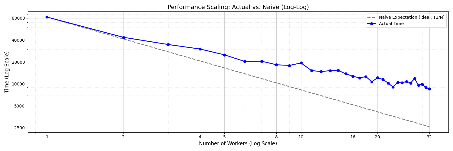
The dashed gray line shows what one would naively expect. The total time required by n workers should equal the time required by one worker, divided by n. The jagged blue graph shows the actual time required by the workers. 32 workers are in fact faster than 1 worker, but only by a factor 10 or so, not by a factor 32. There are several reasons for the discrepancy. The workers do not communicate directly with each other, and there is a delay in making their results available to the other workers. This causes extra work for all workers. There is also a certain overhead in running the workers. The jaggedness of the blue line is due to random effects in distributing parts of the game tree to individual workers and their pruning of their subtrees.

Increasing efficiency ↩

The next line, starting with a button labeled α/β, lets you turn off or modify certain features that increase the efficiency of the algorithm. They are explained in detail elsewhere, here is a quick summary:

α/β pruning: every board position has a numerical score. White tries to pick moves that maximize the score, and Black tries to minimize the score. If White has analyzed the game tree to the point that it knows it can obtain a score of at least α = 100 with its next move, and it examines a node for which it knows that Black at that node can get a score of at most β = 50, then White will never consider making a move leading to that node, because Black will never allow White to go there. White can, and will, ignore the part of the game tree rooted at that node. This kind of pruning saves massive amounts of computations. If there are several possible moves leading to different positions, but with the same maximum score, pruning may affect the final position, and the corresponding move, but not the score of that position.
You can use this button to turn off α/β pruning. But you would want to do this only to impress yourself or your friends with the phenomenal effectiveness of α/β pruning.
Transposition Table . Most board positions can be attained in more than one way. A transposition table keeps track of positions that have already been visited and makes it possible to utilize the analysis already applied to that position at an earlier stage. The button labeled TT lets you turn off the internal transposition table. You may want to do this when using the JavaScript engine. JS handles arrays inefficiently (unlike C++) , and a browser can be stingy with memory allocations. Managing the TT can lead to memory problems and even crash your session.
The text field labeled TT(m) lets you specify the size of the TT in millions of nodes. Increasing it makes the code more efficient, and also increases the risk that it will run into memory problems.
The Opening Book. It seems pointless to recompute the first few moves every time you play a game, particularly since, to paraphrase Horatio Nelson, during the first four plies you cannot go far wrong by placing your piece on any empty four-way intersection. An opening book is a table that tells for a number of early game positions which move to make at that position. The opening book that comes with the code is small, it covers only the first four plies of the game. There are 479 of them, and the moves to be taken for each of them were computed at depth 8. You can compute your own opening book, but it will take a long time, and you will need to keep your browser window open and visible during that time. To use your own book you’ll need to download the files for this page and place them onto a web server that you have access to. To create your own book select the initial number of plies and the depth at which the moves are computed. Clicking on the button labeled create OB will compute the book and download a file named millOB.json to your system. Place it in the same directory that contains your HTML files.
Symmetry: There are some obvious symmetries in the Mill Board. For example, a rotation by 90 degrees does not change the layout of the board. In fact there are only four truly distinct options for making the first move: play on a four way intersection (5, 11, 14, or 20), play on a three way intersection (2, 8, 10, 12, 13, 15,17, 23,19, 21), play on a corner (1, 3, 7, 8, 16,17, 22, or 24) or play on one of the interior corners 4, 6, 19, and 20. It turns out that there are a total of 16 symmetry transformations that do not change the layout of the board. For the first move, clearly it should suffice to investigate only one position in each set. The advantages of symmetry diminish as the game proceeds and the board position gets more complicated, and less symmetric. Keeping track of symmetry is computationally expensive. (The system applies all 16 similarity transforms to each board position obtained by making a single ply, computes a hash code of the resulting position, takes note of the smallest of those codes, and then sees if that code has occurred previously.) Thus you may wish to reduce the number of plies where symmetry is being taken into account. In the text field labeled S: you can set the ply at which the code stops using symmetry to find the best move. The maximum possible choice for that cutoff is 19, which is also the default. In that case the code will take advantage of symmetry during the entire initial placement phase, i.e., the first 18 plies of the game. Setting it to zero will make sure the computer never uses symmetry.

The following Table illustrates the effectiveness of these features. It shows the number of nodes investigated while computing the first move at depths two through 12. The first column lists the depth of the search. The second column, headed none shows the number of nodes in the search tree. This is smaller, but very close to, the number of nodes encountered when searching without any aid. These numbers are computed assuming no mills were formed during the first 6 moves, rather than obtained by running the code. The third column, headed S, shows the number of nodes examined utilizing only symmetry. The last two entries in that column are conservative (aiming for under- rather than overestimating) estimates. The fourth column, headed S+α/β shows the number of nodes obtained by using Symmetry and α/β pruning. The last column, headed S + α/β+TT, shows the counts for using all three facilities, symmetry, α/β pruning, and a transposition table (with a capacity of 16,000,000 positions, divvied up among 30 workers).

Depth	none	S	S+α/β	S+α/β+TT
2	576	192	192	192
4	267,744	44,624	10,428	5,859
6	102,277,344	17,447,118	924,851	648,947
8	31,500,832,224	6,010,574,862	36,747,175	11,753,982
10	7,622,973,656,544	1,800,000,000,000	1,072,674,057	164,095,689
12	1,402,556,105,125,344	540,000,000,000,000	27,450,718,752	3,587,306,472

Note the extraordinary effectiveness of α/β pruning. Using symmetry, for depth 10, it reduces the number of nodes by a factor of approximately 17,000. For depth 12, the corresponding factor is almost 20,000, and it is amplified by a factor 8 using the Transposition Table. For the last entry in the last row, my computer really did visit three and a half billion nodes, at the blistering rate of about 16 million nodes a second.

AI players ↩

The next few rows let you play tournaments of AI players, edit AI brains, and start a simulated evolution of an individual AI player. Recall that the computer algorithm traverses the game tree and assigns scores to the game positions at the leaves of the tree.

Static evaluations ↩

The formula for that static evaluation is

V = - W_GS × ΔGS + W_N3 × ΔN3 + W_N4 × ΔN4 + W_M1 × ΔM1 + W_M2 × ΔM2 + W_FB × ΔFlyBonus
+ W_PD × ΔPD + W_Mill × ΔMill + W_DM × ΔDM + W_NMF × ΔNMF + W_NMR × ΔNMR + W_NMG × ΔNMG

The variables W_subscript represent the weights (or importance) the AI assigns to different aspects of the game. For example, a brain with a high W_M1 will play aggressively for open space, while one with a high W_PD will prioritize capturing pieces above all else.

The Δ in this formula indicates the difference between the corresponding number for White and Black.

The specific parameters used in the formula are:

GS (Group Score): This is the number of groups of a player’s pieces such that no member of one group can visit a member of another group by moving along empty squares or a vertex occupied by a piece of the same color. It provides a measure of fragmentation. The AI is penalized (hence the minus sign) for having its stones scattered into disconnected groups of pieces that cannot support each other.
N3 (Node 3): The number of pieces sitting on a three way vertex.
N4 (Node 4): The number of pieces sitting on a 4-way intersection.
M1 (Mobility 1): The sum of the number of empty neighbors of each piece.
M2 (Mobility 2): The sum of the number of empty vertices that a piece can reach in two moves.
FB (FlyBonus): A bonus applied if the player has exactly 3 stones (the "Flying" phase), reflecting their sudden ability to fly anywhere.
PD (Piece Difference): The number of pieces.
Mill: The number of active mills currently on the board.
DM (Double Mill): The number of double mills, which allows for forming a mill on every turn.
NMF (Near Mill Filled): Two pieces in a line where the third spot is occupied by the opponent but can be captured.
NMR (Near Mill Ready): Two pieces in a line where the third spot is empty (a potential mill).
NMG (Near Mill Guaranteed): Two pieces in a line where the third spot can be occupied in the next move, without the opponent being able to prevent it.


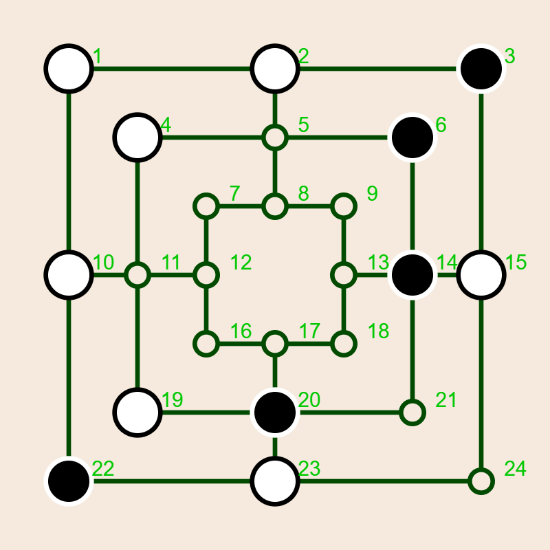
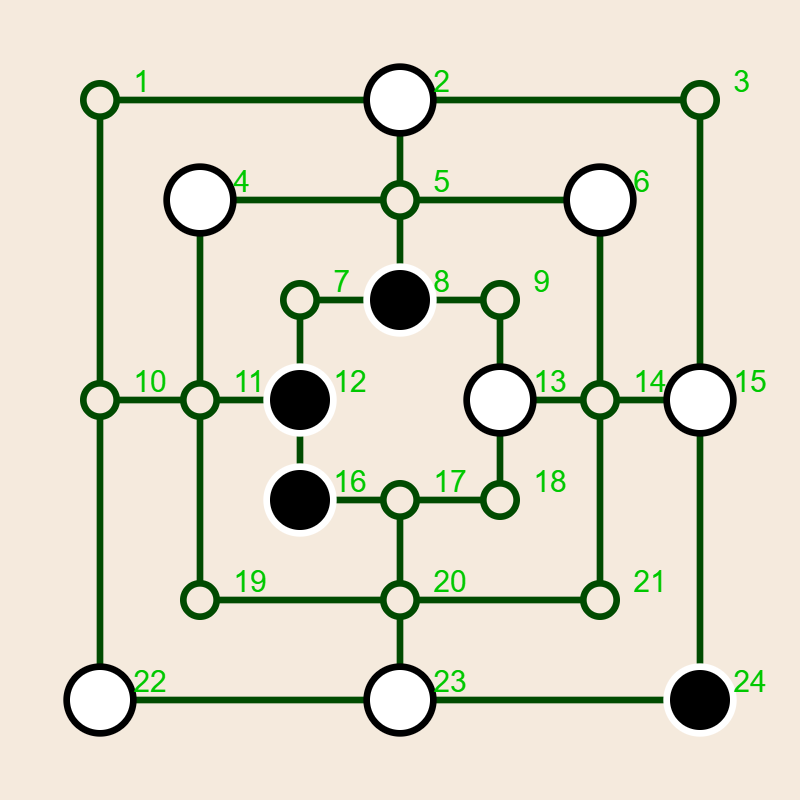
Group score	Double mills	Double mills	Near mills

These concepts are illustrated in the four boards above. On the leftmost board, both Black and White have two separated groups of pieces. One of White’s groups consists of the stones on 15 and 23, and one of Black’s groups consist of the single piece on 22. In both cases the remaining pieces form the second group. There are three kinds of double mills, illustrated in the middle two boards. In the second board, White can move the piece on 23 up and down, and Black can move its piece on 9 back and forth. In board 3, White can move its piece on 4 up and down. Each of those moves closes a mill. The concept of a near mill is illustrated in the fourth board, on the right. The points {22, 23, 15} contribute to NMF, the points {2,4,6} to NMR, and the points {6, 13, 15} to NMG. Black also has a near mill contributing to NMG.

The following table lists the specific weights assigned to the different AI personalities defined in the software. These values determine the strategic character of each player.

Name	GS	N3	N4	M1	M2	FB	PD	Mill	DM	NMF	NMR	NMG
Arwen	62	13	33	178	4	78	552	18	1000	10	98	626
Bilbo	47	13	31	153	4	33	480	24	1000	12	52	531
Celebrian	79	16	48	184	4	92	733	22	1000	10	116	713
Dwalin	37	11	29	145	3	30	452	24	1000	15	54	508
Eowyn	81	15	49	267	4	89	741	28	1000	12	57	856
Frodo	55	13	32	162	4	56	516	21	1000	11	75	579
Galadriel	50	15	30	10	4	300	1000	100	500	10	20	30
Hamfast	1000	1000	1000	1000	1000	1000	1000	1000	1000	1000	1000	1000
Indis	0	0	0	0	0	0	0	0	0	0	0	0
Jolly	-62	-13	-33	-178	-4	-78	-552	-18	-1000	-10	-98	-626

The weights are normalized so that the maximum weight is 1000. The players are sorted roughly by decreasing playing ability.

You may recognize the names of the brains which replace the standard Alice, Bob, ... sequence. When first starting to create the AI players I guessed some suitable parameters which are now Galadriel's parameters. The parameters of the first AI player were all created, going back to Galadriel in some way or other, by the evolution algorithm that is part of the software. Frodo's parameters are the average of Arwen's and Bilbo's parameters.

The last three players were added for fun and for experimental purposes. Hamfast says that all these factors are important but he can’t bother distinguishing them, Indis says that she is too busy paying attention until she recognizes a certain win or loss in her subtree, and Jolly is in love with Arwen and will do everything he can to help her win.

Silence is golden ↩

Returning to the controls in the middle column of the Game Page, the next row contains only one button, prominently labeled Silence, on or off. If silence is off each game in a tournament or an evolution cycle will be displayed on the game board. Otherwise only the status window will contain information about the progress being made. You can turn silence on or off temporarily as the tournament or improvement cycle proceed. With silence on the tournament or improvement cycle will proceed faster.

Whether you do or do not display the games, keep in mind, however, that browsers typically limit the access of a page if the page is not at least partly visible on the screen. So if you want to run a tournament or an evolution overnight make sure your computer stays on and the board shows on the screen.

Dealing with brains ↩

The next three rows let you improve (or impair) a brain, and import or export your own list of brains.

Modifying a brain ↩

You can freely modify the built-in brains. To do so select the brain you want to modify, using the menu labeled brain. You will see the weights for that specific brain. To modify them just enter the new value. Your modifications will be active until you exit the Game Page.

Brain improvement ↩

You can attempt to improve a brain using the built in genetic algorithm. It proceeds by applying a small random change to a brain, and running a tournament between the player and its mutant. If the mutant wins the AI then tries to refine that mutation with a line search in the direction of the change, and finally replace the player with the mutant when the line search converges. If the current player wins the initial tournament the AI applies another random change (a new generation) and runs another tournament. Note that if a parameter is set to zero then it cannot be changed because mutations add or subtract a percentage of the current value.

To run the evolution proceed as follows:

Select a Brain: Choose a brain from the menu labeled Brain to edit or improve.
In the first text field to the right of the Brains Menu, pick the number of generations. This choice is not critical, since any successful mutation is uploaded and saved as soon as it is found. So you can interrupt the ongoing evolution at any stage without losing any information.
In the next text field, set the number of games in the tournament. The AI will play that number of games twice, once with the mutant being White, once with it being Black. 10 games strike a reasonable balance between reliability and efficiency.
In the rightmost Percent: Set Max percentage change. For refinements of an existing successful brain 5% is a good choice. If you start with a very rough approximation you can choose a higher percentage. The applied percentage may be adjusted by the system as the evolution proceeds.
Start: Click on the button labeled Improve.
Once an improved mutation is found the AI will download a JavaScript file defining the mutation, and suitable for pasting into a JS code. The file will appear where your downloads usually appear, e.g., in your Downloads folder.

Import/export brains ↩

The next line lets you import or export a comma delimited spreadsheet with a specified list of brains Thus you can keep your own list of players without having to edit them each time you play. To do so enter the filename (without the .csv extension) in the text field labeled brains and click import or export. Export will put the file into your download directory. Clicking Import will look for the file on the server. If it cannot find it the code will open a dialog where you can specify the location of your brains list. As an example, here is the spreadsheet with the built-in brains.

Running a tournament ↩

The next three lines let you design and run a tournament. To do so follow these steps:

Select the search depth for the games, using the two menus labeled Time below the status window. You can choose time mode as well but keep in mind that time means wall clock time and that the game will run much more slowly when the Game Page is invisible, for example, when you temporarily use your computer for other purposes. I usually run tournaments at depth 6. You can have different search depths for White and Black.
Choose the number of games played by each pair of players. Keep in mind that there is a great deal of randomness in the moves made by the players, and that most games are draws. If you really want to know which players are better choose a large number like 100 games per pair.
Choose the participants using the selection buttons labeled with the first letters of the players’ names.
Click on run tournament.
The code will have each player play the specified number of games, once as Black and once as White, against every other player. When the tournament is over it will upload a comma delimited spreadsheet to your computer. You can see the results of a depth 6 100 game tournament among the player listed here. The ordering of the computer brains is based on that tournament, rather than vice versa. The names of the computer brains were assigned after the tournament.

Setting up a board ↩

The next to last row in the second column lets you create specific board scenarios for computer analysis. Start by clicking on the setup board button. This will interrupt any ongoing game and change the color of the board. The current board state remains unchanged. You can then click on any vertex and cycle through the three possible states (White, Black, empty) of that vertex. The ply number in the text field next to the setup button determines whose play (even is White, odd is Black) it is, and whether the game is in the placement (ply count ≤ 18) or moving phase (ply count > 18). If you just want to continue the game you don’t need to do anything. However, you can change the current ply number by entering its new value in the text field. To finish the set up process click again on the setup board button.

As mentioned above, the last row lets you create an opening book.

Switching engines ↩

The remaining controls are located in the third column of the Game Page. The first row lists the version number and the engine of the code. This is actually a button that lets you switch the engines. I originally started writing this software entirely in JavaScript. JavaScript is the language of choice for designing interactive web pages. However, letting the parallel worker calculations be handled by compiled C++ code makes the game much more efficient. You want to use the C++ engine if you can, and use the JS version only if you have to, or if you want to compare the performances of the two engines.

Playing and resetting ↩

The next row contains the Play button. Use it to start a game, or to interrupt a game, tournament, or improvement cycle.

The Reset button in the next row resets the board to its original position. It has no effect on other settings.

The game table ↩

At the bottom of the third column is the Game Table. It lists the moves as they happen. Each row of that table lists

In the column headed n, the number of the ply. The Game Board shows the status after that ply is applied.
The column headed P lists the player whose move it is. This is actually a button. Clicking on it will interrupt the game if it is ongoing, and will display the board state after that particular ply. You can then step through the game using the Forward and Backward Buttons above the game table, change player parameters, or modify the board. You can resume the game, with the changes applied, by clicking on the Play button.
The action of that ply is described in the next three columns, headed by p, q, and x. p denotes the vertex where a stone was placed or a move was started. If the action is an actual movement, q denotes the destination of the moved stone. x denotes the location of any opposing stone that is removed.
The columns headed w and b contain the numbers of White and Black pieces after the ply.
The last column of the game table gives the static evaluation of the board after the ply. Recall that you can obtain a deeper level evaluation by using the Evaluate Board button.